Designing a Balcony HF Magnetic Loop Antenna - Part 1
#magloop #antenna #hf #balcony #urban #nec2 #diy #qrp #homebrew #modelling #theory
Reading time: 35 minutesThis post has been a long time coming, and is my understanding of the commonly termed magnetic loop antenna. I invite people to please let me know if there are issues with my understanding, the TLDR; version:
- Constraints to deploy at my QTH
- Current flow and LC Circuit of a loop antenna
- Choosing a shape for the antenna
- What bands should I build it for?
- Materials and construction choices in terms of copper, and frame
- Some elementary calculations to consider for the build
Balcony Operating Constraints
Operating a HF station in an urban Indian environment is tricky (at best)! Previously, when I was operating from my QTH, I used to throw a wire outside the window using a telescopic fishing pole. However, this is highly sensitive to nearby concrete rebar, wind and metal railings, each of which tends to detune the system in an unpredictable manner. This structural proximity causes the SWR to change inconsistently across bands, limiting operations to late-night hours when the ground below is vacant and requiring a tedious, 30-minute setup and tear-down sequence. Operating from a 5th-floor balcony (without access to the terrace) in a dense residential neighbourhood like Bangalore immediately rules out traditional full-sized wire dipoles or quarter-wave verticals, which require expansive outdoor real estate. Consequently, a self-contained, quiet balcony antenna, with an acceptable performance1, becomes an absolute necessity.
- Rebar- Shielding and Detuning: In India, multi-storey apartment buildings are constructed of heavily reinforced concrete. From an electromagnetic standpoint, this dense grid of steel reinforcing rebar acts as a lossy, reflective Faraday shield. Placing an antenna inside or directly against the balcony floor and ceiling significantly dampens signals and heavily attenuates both receive and transmit performance. Even if the steel is not a “dense” grid, it still detunes the antenna and adds loss!
- Urban QRM Floor: Densely populated urban environments suffer from an exceptionally high floor of man-made electromagnetic interference (QRM). This localised electrical noise is continuously emitted by switched-mode power supplies (SMPS), cheap LED lighting, and consumer household electronics, resulting in a persistent S-meter noise floor of S7 to S9 on traditional wire antennas (at some point I’d like to give you folks measurements for it).
- Compliance & Portability Mandate: To remain compliant with strict rules of the apartment association2, any antenna installation must be completely within the balcony with nothing protruding beyond the balcony railing. Nothing can be permanently fixed to the railing or the balcony, so the antenna must be quick to set up and take down, and even while deployed it must pose no risk to residents below.
- Radios and Power: The loop needs to work with my QMX, zBitx and sBitx, so it must handle 5–10 W comfortably and up to about 25 W with the sBitx. Which bands to target is something I’ll work out from the numbers later in this post as we go along. Since we are working QRP mostly, my design should work with it, but the challenge with loops is that the tuning capacitor has to withstand about 2–3 kV at 10 W, and over 4 kV at 25 W, on 40 m (we shall see the calculation in the later sections).
Please note that I have used LLMs to create the scripts to generate the images in this post. They serve as good ways for me to understand the theory of antennas, and creating cleaner images than drawing them by hand is a good choice for this kind of post.
Theory
Near-Field Physics: Electric vs. Magnetic Coupling
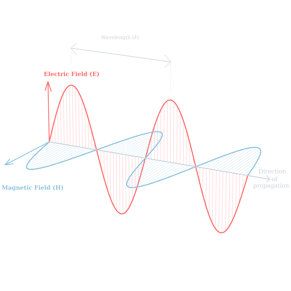
Figure 1: 3D vector representation of propagating electromagnetic wave showing orthogonal E and H fields.
According to classical electrodynamics, time-varying electric (\(E\)) and magnetic (\(H\)) fields are inherently coupled. In a transmitting antenna both fields are established simultaneously as co-existing components of an electromagnetic wave.
Typically, antennas are classified based on the dominant type of reactive energy stored in their immediate vicinity:
- Electric Antennas (e.g., a short dipole) store energy primarily in an electric field (\(E\)) in the near-field region, behaving as a highly capacitive circuit element.
- Magnetic Antennas (e.g., a small loop) store energy primarily in a magnetic field (\(H\)) in the near-field region, behaving as a highly inductive circuit element.
What is the near-field region? The space around an antenna is usually divided into three regions, two of which make up the near-field. \(D\) is the largest dimension of the antenna, \(λ\) is the wavelength and \(r\) is the distance from the antenna, in the equations below:
- Reactive near-field region: The region immediately surrounding the antenna where the reactive (non-radiating) fields dominate. The boundary is defined as:
For an electrically small antenna (\(D \ll \lambda\)), such as the small loop antenna we wish to design, this boundary is commonly taken as the radian distance:
\begin{equation} \label{eq:reactive\_nearfield\_small} r < \frac{\lambda}{2\pi} \approx 0.159\lambda \end{equation}- Radiating near-field (Fresnel) region: The region where radiation fields begin to dominate, but the angular field distribution is still dependent on the distance from the antenna. The boundaries are:
Note: This region may not exist if the antenna is electrically small relative to the wavelength (as is the case with our design).
- Far-field (Fraunhofer) region: The region where the angular field distribution is completely independent of the distance. The radiation pattern is fully formed, and the waves behave as local plane waves. The boundary is defined by:
Subject to the additional constraints of \(r \gg D\) and \(r \gg \lambda\).
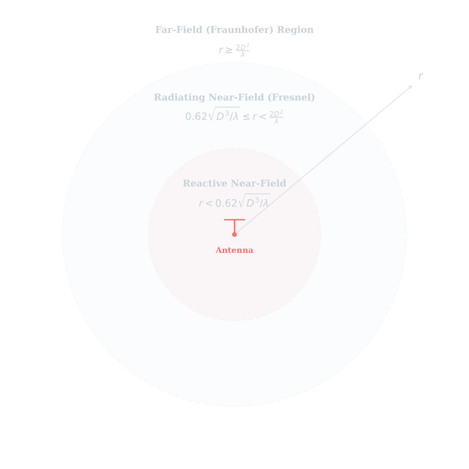
Figure 2: The three field regions surrounding an antenna based on radial distance.
So what does this mean for a balcony loop? Looking at the table below3, there is no band where I can get the antenna “away” from its surroundings. Even on 10 m the reactive near-field reaches out about 1.7 m, and on 40 m it is close to 7 m. Either way, the railings, the rebar in the slab and every charger and LED driver in my flat (and probably my neighbour’s) are well within it. This cuts both ways. On the plus side, it is exactly why a magnetic loop makes sense here: it is far less bothered by the local electric-field noise that a wire antenna happily soaks up, and the lower the band, the more of that noise sits in the near-field. On the minus side, the loop’s strong magnetic near-field will couple into all that nearby steel, including the rebar inside the concrete, and lose power there, so where I place it on the balcony matters a lot. In short, from a near-field perspective the loop helps on every band; which bands it actually works well on comes down to its size and efficiency, which I’ll work out in the calculations section below.
| Band | Lower edge (MHz) | Upper edge (MHz) | \(\lambda\) at lower edge (m) | Reactive near-field \(\lambda/2\pi\) (m) |
|---|---|---|---|---|
| 160 m | 1.800 | 1.825 | 166.6 | 26.5 |
| 80 m | 3.500 | 3.900 | 85.7 | 13.6 |
| 60 m | 5.3515 | 5.3665 | 56.0 | 8.9 |
| 40 m | 7.000 | 7.200 | 42.8 | 6.8 |
| 30 m | 10.100 | 10.150 | 29.7 | 4.7 |
| 20 m | 14.000 | 14.350 | 21.4 | 3.4 |
| 17 m | 18.068 | 18.168 | 16.6 | 2.6 |
| 15 m | 21.000 | 21.450 | 14.3 | 2.3 |
| 12 m | 24.890 | 24.990 | 12.0 | 1.9 |
| 10 m | 28.000 | 29.700 | 10.7 | 1.7 |
| 6 m | 50.000 | 54.000 | 6.0 | 1.0 |
In a typical urban apartment, depending on the source of the man-made noise (QRM), either the \(E\)-field or the \(H\)-field can dominate. A wire antenna is an electric antenna, so it couples strongly to local E-field noise. Its feedline, which runs through the same near-field, adds common-mode noise on top of that4.
Conversely, an electrically small, balanced loop antenna operates as a magnetic dipole. In its near-field region (less than \( \lambda/2\pi\)), the loop responds mainly to the magnetic (H) field component of the local field. The reasons are simple: it picks up less local \(E\)-field noise; being balanced, it picks up far less common-mode noise via the coax; its narrow bandwidth admits less noise; and we can rotate a null towards a noise source. In this case, it’s the signal-to-noise ratio that matters, not the S-meter reading. Operators commonly report a noticeably lower noise floor, sometimes 10 dB or more5. Since the loop is less efficient, signals drop too, so this is something to consider when using a loop antenna.
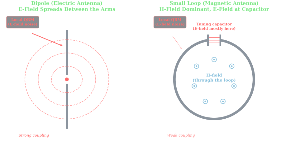
Figure 3: Near-field coupling to local electric-field noise: a dipole’s E-field spreads out between its arms and couples strongly to nearby noise, while a small loop is H-field dominant, with its E-field mostly confined to the tuning capacitor.
Furthermore, as a high-Q resonator, the magnetic loop acts as a sharp, highly selective bandpass preselector directly ahead of the receiver’s front-end. With an extremely narrow instantaneous SWR bandwidth (only a few kHz on 40 m), it heavily attenuates strong out-of-band broadcast signals, preventing receiver desensitisation and front-end overload. However, it does mean it needs retuning every few kHz because of the narrow bandwidth.
It is vital to clarify a common electromagnetic myth: that a ‘magnetic’ loop radiates or receives only the magnetic field. Once a radio wave propagates into the far-field (beyond a wavelength or so), the ratio of the \(E\)-field to the \(H\)-field is permanently fixed at \(120\pi\) or 377 Ohms (the intrinsic impedance of free space). Therefore, in the far-field, both dipoles and loops generate and respond to both components identically. However, because the loop’s near-field \(E\)-field is mostly concentrated around its tuning capacitor, it puts much less electric field into the surrounding ground and concrete, so it loses less there than a low wire antenna would, and works reasonably well even when mounted low or in compromised spaces. Its magnetic near-field still couples into nearby steel, though, so it is not loss-free. In practical terms, that concentrated E-field means over 2.5 kV across the tuning capacitor even at 10 W on 40m (see the calculations below), which is enough to give a nasty RF burn.
The Uniform Current Assumption
Textbooks treat a loop as electrically “small” when its circumference (\(C\)) is below about \(\lambda/10\), because the current around it is then practically uniform6. In practice, hams use loops up to about \(\lambda/4\) on their highest band (some go up to about \(\lambda/3\)), and much below \(\lambda/10\) the efficiency drops off sharply. The practical sweet spot is therefore roughly \(\lambda/8\) to \(\lambda/4\)7. The fundamental operating principle of the loop relies on the Uniform Current Assumption.
When the current is (nearly) uniform:
- The amplitude and phase of the alternating RF current remain virtually uniform and in-phase at all points along the loop conductor.
- The loop behaves as a magnetic dipole, with its axis perpendicular to the plane of the loop.
- The radiation pattern is a doughnut lying in the plane of the loop, with deep, sharp nulls straight through its face. For a vertical loop, this means equal radiation in every direction within the plane of the loop, a figure-8 when seen from above, and vertical polarisation at low angles. Those nulls are handy: rotating the loop can point one at a noisy neighbour.
If the loop’s circumference grows beyond about \(\lambda/4\):
- The current distribution along the conductor becomes increasingly non-uniform.
- The phase of the current shifts at different points along the conductor.
- Somewhere past about \(\lambda/3\), the nulls start to fill in and the pattern distorts. At about \(1\lambda\), it becomes a full-wave loop (like a quad or delta-loop element), and the pattern flips by 90°: maximum radiation now goes straight through the face, exactly where the small loop had its nulls.
Thus, keeping the loop between about \(\lambda/8\) and \(\lambda/4\) on the bands we care about, and no more than about \(\lambda/4\) on the highest one, preserves its predictable pattern, its nulls and its quiet near-field behaviour.
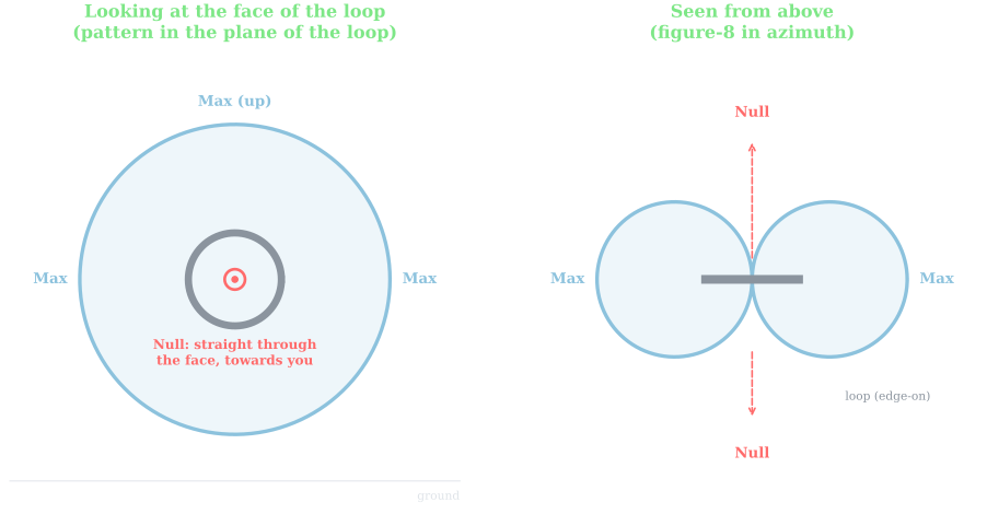
Figure 4: Free-space radiation pattern of a vertical small loop. Face-on, it radiates equally in every direction within the plane of the loop; seen from above, it is a figure-8 with deep nulls straight through the face. Near the ground and a building, the real pattern will be distorted.
To see what this means in practice, the table below shows how “big” a 1 m × 1 m square loop (\(C = 4\) m) is on each band. It sits in the \(\lambda/8\) to \(\lambda/4\) sweet spot from 30 m to 17 m, is slightly over \(\lambda/4\) on 15 m, is just below \(\lambda/10\) on 40 m, and stops being a small loop altogether by 10 m. Efficiency will decide how far down we can realistically go, which we’ll calculate later.
It would be wonderful to check real-world propagation with the loop mounted vertically and horizontally!
| Band | \(C/\lambda\) (lower edge) | \(C/\lambda\) (upper edge) | Verdict |
|---|---|---|---|
| 160 m | 0.024 | 0.024 | Far too small, very inefficient |
| 80 m | 0.047 | 0.052 | Too small, very inefficient |
| 60 m | 0.071 | 0.072 | Small, inefficient |
| 40 m | 0.093 | 0.096 | Just below λ/10, works but lossy |
| 30 m | 0.135 | 0.135 | Sweet spot |
| 20 m | 0.187 | 0.191 | Sweet spot |
| 17 m | 0.241 | 0.242 | At λ/4, the upper limit |
| 15 m | 0.280 | 0.286 | Just over λ/4, still usable |
| 12 m | 0.332 | 0.333 | λ/3, pattern distorting |
| 10 m | 0.374 | 0.396 | Too large |
| 6 m | 0.667 | 0.720 | Not a small loop any more |
The Resonant LC Circuit & Mutual Inductance Model
Electromagnetically, a transmitting magnetic loop is not merely a radiator; it is a resonant LC (tank) circuit8. The same large current flows through the loop and the capacitor, and every loss can be modelled as a small resistance in series with them. This gives the following equivalent circuit:
- The Inductor (\(L_2\)): The main outer loop conductor acts as a high-Q, single-turn inductor. Its inductance is determined by the physical perimeter/shape of the loop and the cross-sectional diameter of the conductor. A 1 m × 1 m square of 22 mm copper tube is about 3 µH.
- The Capacitor (\(C\))9: A tuning capacitor connected across a gap in the loop (usually at the top) closes it into a resonant circuit. It can be an air-variable, butterfly or vacuum capacitor, or a home-made sliding-tube “trombone”. It sets the resonant frequency, \(f = 1/(2\pi\sqrt{LC})\).
- The Coupling Loop (\(L_1\)): A smaller loop, often a shielded (Faraday) loop, though a plain wire loop also works, sized at about \(1/5\) of the main loop as a starting point and then adjusted for the best SWR. It is connected directly to the 50 Ohm coaxial transmission line 7. Sited opposite the tuning capacitor, it has no physical electrical connection to the main loop. Instead, it acts as the primary winding of an air-core transformer, inductively transferring RF energy to the main loop through Mutual Inductance (\(M\)). In doing so, it transforms the loop’s tiny resistance up to about 50 Ohms.
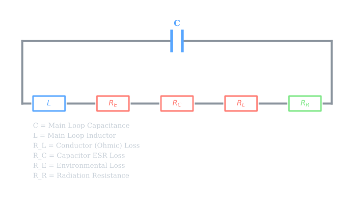
Figure 5: Equivalent circuit of the main loop: inductor and tuning capacitor with the conductor, capacitor, environmental and radiation resistances in series.
Because of the loop’s electrically small size, its radiated power is represented by an incredibly tiny Radiation Resistance (\(R_R\)). On the 40m band (7 MHz), a 1 m × 1 m square loop has a radiation resistance of only about \(0.009\ \Omega\). To maximise overall antenna efficiency, we must minimise all other series loss resistances in the loop damping equation:
\begin{equation} \label{eq:total\_damping\_loss} R\_{\text{Total}} = R\_L + R\_C + R\_E + R\_R \end{equation}Where:
- \(R_L\) (Conductor Loss): The ohmic resistance of the main loop tubing. Due to the RF skin effect, current is forced to flow only within the outer few tens of micrometres (about 25 µm in copper at 7 MHz) of the conductor surface. To minimise \(R_L\), we must use highly conductive, large-diameter round tubing (such as copper or aluminium) and make every joint a low-resistance one: soldered, brazed or firmly clamped.
- \(R_C\) (Capacitor Loss): The equivalent series resistance (ESR) of the tuning capacitor and its joints 10. High-Q loops carry large circulating currents: over 20 A on 40 m at 25 W for our loop. Any mechanical sliding “wiper” contacts in standard capacitors introduce high contact resistance. Using a split-stator (butterfly) capacitor (the loop connects to the two stators, and the current passes from one stator to the other through the rotor, with no sliding contact) 11 or a sliding-tube ‘trombone’ capacitor12, or a vacuum variable, avoids these contact losses.
- \(R_E\) (Environmental Loss): The loss resistance induced when the loop’s intense near-fields couple inductively to nearby lossy objects, such as reinforcing steel rebar in concrete balcony walls. A common rule of thumb is to keep the loop at least one loop diameter away from large metal objects. Steel is the worst, but any metal causes some loss.
- \(R_R\) (Radiation Resistance): Not really a loss at all. It represents the power that leaves as radio waves, which is the part we want. Efficiency is simply \(\eta = R_R / R_{\text{Total}}\).
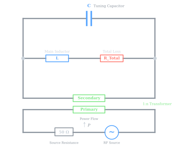
Putting it together: the transmitter drives the coupling loop, which is magnetically coupled to the main loop. At resonance, the reactances of \(L\) and \(C\) cancel, leaving only \(R_{\text{Total}}\), a fraction of an Ohm, and the coupling loop transforms this to about 50 Ohms. That is why changing the size, shape or position of the coupling loop is how you fine-tune the SWR.
Practical considerations
Choosing the Bands: 40 m to 15 m
Before choosing a shape or a construction method, I need to decide which bands the loop has to cover, because that sets everything else: the size of the tuning capacitor, the voltage it must survive and how fat the conductor needs to be. Three things decide the bands for me: what my licence allows, what a loop of this size can do well, and what I actually want to do on the air.
- What my licence allows: with a Restricted Grade licence, I can use 160, 80, 40, 20, 17, 15, 12 and 10 m at up to 50 W. 60 m and 30 m are not available to me (see the band table and its footnote earlier).
- What the loop can do well: from the electrical-size table, a 1 m × 1 m square sits in the \(\lambda/8\) to \(\lambda/4\) sweet spot from 30 m to 17 m. It is slightly over \(\lambda/4\) on 15 m, and just below \(\lambda/10\) on 40 m, where it still works but is lossy.
- What I want to do: mostly QRP, with the occasional DX contest.
Putting these together, each band earns its place for a different reason:
- 40 m: the band for domestic and regional contacts and for POTA activity in India. A small loop is inefficient here, but the band is too useful to leave out.
- 20 m: the everyday DX workhorse, open most days, and a contest band. It is also right in the loop’s sweet spot.
- 17 m: quieter, and good for QRP DX. It is a WARC band, so there are no contests on it, but that is part of its charm.
- 15 m: daytime DX and a contest band. The loop is slightly over \(\lambda/4\) here, but still usable.
Together, 40, 20 and 15 m also cover the contest bands I am realistically likely to use.
And the bands I am leaving out:
- 160 m and 80 m: far too small electrically. Even built from 22 mm copper tube, a 1 m square would radiate only about 2% of the power on 80 m and about 0.2% on 160 m.
- 12 m and 10 m: the square is past \(\lambda/3\) on 12 m and well beyond it on 10 m, so it no longer behaves like a small loop, and both bands depend heavily on the sunspot cycle, which is now past its peak. If the loop happens to tune there, it is a bonus, not a design goal.
One consequence of this choice is worth flagging now: 7.000 to 21.450 MHz is roughly a 3:1 frequency range. Since the capacitance needed goes with \(1/f^2\), the tuning capacitor has to cover roughly a 9:1 or 10:1 range, plus a little margin for stray capacitance. One good variable capacitor can do this, and the calculations section sizes it.
Finally, power: the QMX and zBitx give me 5–10 W, and the sBitx up to about 25 W, all comfortably under the 50 W limit of my licence. As the calculations will show, it is the capacitor voltage, not the licence, that makes 25 W the hard part.
Choosing the Shape
A magnetic loop does not have to be round. Electrically, only two things about the shape matter: the area it encloses, because the radiation resistance goes up with the square of the area, and the length of conductor, because that sets the conductor loss. So I compared five shapes in two ways: first with the same area (1 m²), then with the same length of tube (4 m, enough for a 1 m × 1 m square). All the numbers assume 22 mm copper tube and conductor loss only, as in the calculations section.
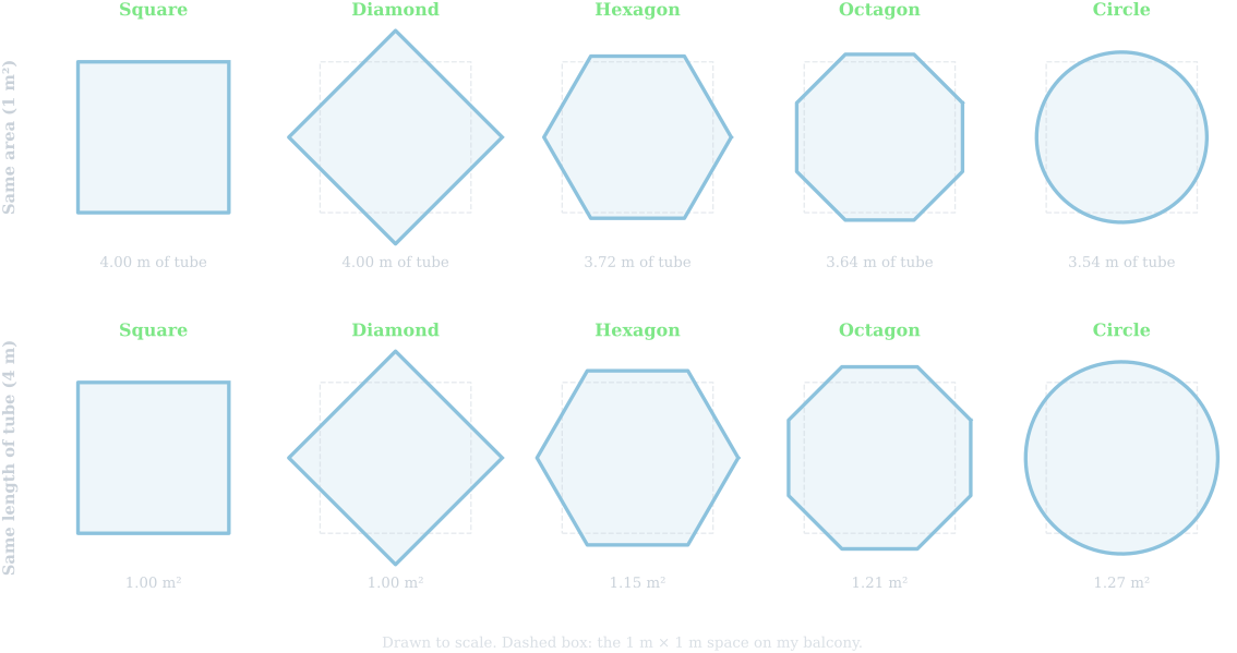
Figure 6: The five shapes, drawn to scale, with the same area (top) and the same length of tube (bottom).
Same area: 1 m²
| Shape | Size | Footprint (m) | Tube needed (m) | 40 m | 20 m | 15 m | Reaches \(\lambda/4\) at | Joints |
|---|---|---|---|---|---|---|---|---|
| Square | 1.00 m sides | 1.00 × 1.00 | 4.00 | 20% | 73% | 92% | 18.7 MHz | 4 × 90° |
| Diamond | 1.00 m sides | 1.41 × 1.41 | 4.00 | 20% | 73% | 92% | 18.7 MHz | 4 × 90° |
| Hexagon | 0.62 m sides | 1.24 × 1.07 | 3.72 | 21% | 75% | 92% | 20.1 MHz | 6 × 60° |
| Octagon | 0.46 m sides | 1.10 × 1.10 | 3.64 | 21% | 75% | 93% | 20.6 MHz | 8 × 45° |
| Circle | 1.13 m diameter | 1.13 × 1.13 | 3.54 | 22% | 76% | 93% | 21.1 MHz | Continuous bend |
With the same area, every shape has the same radiation resistance, so the only difference is how much tube it takes to enclose that area. The circle needs the least, so it has the lowest conductor loss, but the advantage is tiny: at most 2 percentage points, well under 0.5 dB. What changes a lot is the footprint: the square is the only one that fits a 1 m × 1 m space, while the diamond, which is electrically identical to the square, needs a 1.41 m space because it stands on its corner.
Same length of tube: 4 m
| Shape | Size | Footprint (m) | Area (m²) | \(R_R\) vs square | 40 m | 20 m | 15 m | Joints |
|---|---|---|---|---|---|---|---|---|
| Square | 1.00 m sides | 1.00 × 1.00 | 1.00 | 100% | 20% | 73% | 92% | 4 × 90° |
| Diamond | 1.00 m sides | 1.41 × 1.41 | 1.00 | 100% | 20% | 73% | 92% | 4 × 90° |
| Hexagon | 0.67 m sides | 1.33 × 1.15 | 1.15 | 133% | 25% | 79% | 94% | 6 × 60° |
| Octagon | 0.50 m sides | 1.21 × 1.21 | 1.21 | 146% | 26% | 80% | 94% | 8 × 45° |
| Circle | 1.27 m diameter | 1.27 × 1.27 | 1.27 | 162% | 28% | 82% | 95% | Continuous bend |
With the same length of tube, the shapes enclose different areas, and here the differences are bigger. A circle encloses 27% more area than a square from the same tube, which gives it 62% more radiation resistance. On 40 m, that is 28% versus 20% efficiency, about 1.5 dB. On 15 m, it hardly matters. The catch is that every shape except the square needs more than 1 m of space.
So which shape?
The two tables tell the same story from different sides: the more “round” the shape, the better it uses its tube, but the advantage is at most about 1.5 dB on 40 m and almost nothing on the higher bands. On my balcony, the space is the hard limit, not the tube, and in a 1 m × 1 m space the square encloses the most area. That is why the calculations use a square.
The square has one drawback: its 4 m perimeter passes \(\lambda/4\) at 18.7 MHz, so on 15 m it is slightly beyond the usual limit (about \(0.29\lambda\)). It is still usable, but the pattern will be a little less tidy there.
What each shape means to build
The shape and the construction method are not independent; some combinations are easy and some are a fight:
- Copper tube: square and octagon are straightforward, using standard 90° or 45° plumbing elbows, soldered all round. A circle needs a tube bender, or soft copper AC tubing that already comes in a coil, gently opened out. Hexagons need 60° fittings, which are hard to find.
- Foil on PVC: square and octagon again, using standard PVC elbows. The weak point is carrying the foil continuously around each elbow without gaps, so fewer corners is better, which favours the square. Bending PVC into a circle is possible with heat, but tricky.
- Wire on a frame: any shape is easy. A “+” shaped frame with the wire run around its tips makes a diamond; an “×” shaped frame makes a square; a hula hoop makes a circle. This is also the quickest to fold away.
Choosing the Construction
The loop conductor is where most of the loss happens, so how I build it matters as much as its size. There are three practical options for a home-brewer: copper tube, copper foil on PVC pipe, and wire on a frame. The calculations section puts numbers on each, but the short version is this: the conductor barely matters on 15 m, and matters enormously on 40 m.
All three are limited by the same piece of physics. At RF, current flows only in a thin skin on the surface of the conductor, so what matters is the surface, not the bulk. A fatter conductor has more surface, and so less loss:
| Band | Frequency (MHz) | Copper (µm) | Aluminium (µm) |
|---|---|---|---|
| 40 m | 7.0 | 25 | 32 |
| 20 m | 14.0 | 18 | 23 |
| 15 m | 21.0 | 14 | 19 |
As a rule of thumb, the conductor should be at least two to three skin depths thick. Any solid tube or wire easily meets this; foil may not, as we will see.
Copper tube
This is the classic magloop: rigid copper tube, soldered at every joint.
- Pros: the lowest loss and the most predictable performance. It is rigid, so it holds its tuning, and soft copper AC/refrigeration tube up to 7/8" (about 22 mm) is easy to find in India.
- Cons: it is heavy (around 2 kg for a 1 m × 1 m square of 22 mm tube, before fittings) and the most expensive option. Every joint must be soldered or brazed all the way round; a single poor joint can add more loss than the entire length of tube.
- On the balcony: a rigid 1 m square has to be carried in and out whole each time, so it needs to fit through the door and have somewhere to live indoors.
Aluminium tube is a lighter and cheaper alternative. Its higher resistance costs a little (roughly 30% more conductor loss than copper of the same size), and it cannot easily be soldered, so joints have to be firmly clamped and kept clean.
Copper foil on PVC pipe
Here, the PVC pipe is just a former, and a layer of copper foil on it (or inside it) does the conducting.
- Pros: light and cheap. Because the current only flows on the surface, a large PVC pipe gives a large effective diameter for very little copper, so a well-made foil loop can match, or even beat, a smaller copper tube. With the foil inside the pipe, it is also protected from the weather.
- Watch for the foil thickness: the copper should be at least about two skin depths thick, which is about 50 µm on 40 m. Common copper foil tapes are often only around 35 µm of copper, so two layers, or thicker copper sheet, are safer. Kitchen aluminium foil (around 15–20 µm) is thinner than aluminium’s skin depth on 40 m, so I would avoid it.
- Lay the foil lengthwise, not in a spiral: the current flows along the pipe, so strips laid along its length let it flow uninterrupted. A spiral wrap forces it to cross the adhesive at every turn.
- Joints and seams: solder the overlaps where possible, since conductive adhesive alone adds resistance. Carrying the foil continuously around each elbow is the hardest part, which is another reason to prefer fewer corners.
- Weather: foil on the outside will peel and oxidise in the monsoon and the sun unless it is sealed.
Wire on a frame
The simplest option: a wire run around the tips of a frame made of PVC, wood or fibreglass.
- Pros: the lightest and cheapest, and the frame can be made to fold, so it is the quickest to set up and take down. That fits the “temporary only” rule of my apartment association best.
- Cons: much higher conductor loss, because a thin wire has very little surface. With 2.5 mm² house wire, the calculations show about 3 dB of extra loss on 15 m, but about 10 dB on 40 m.
- Improving it: several wires in parallel, spaced a few centimetres apart, behave like a fatter conductor and recover some of the loss. The braid of a thick coax cable (such as RG-213 or LMR-400) is another popular middle ground.
Common to all three
The joints between the loop and the tuning capacitor carry the full loop current, which the calculations show can exceed 20 A on 40 m at 25 W. Thin wires here can quietly add more loss than the whole loop, so whichever construction I choose, those connections need to be wide copper straps, soldered or firmly bolted.
Since 40 m is one of my target bands, wire is ruled out as the main conductor, which leaves copper tube or foil on PVC. The calculations section below compares all three in detail. I will have to figure out what works best from a construction possibility and modularity to keep changing things when I build this antenna!
Calculations
Time to put numbers on all of this. I have run the calculations for a 1 m × 1 m square loop, the shape that makes the most of my balcony space based on the choice of shape discussed earlier, built in the three ways discussed above: 22 mm copper tube, copper foil on 32 mm PVC pipe, and plain 2.5 mm² house wire on a frame. Each table below has the three builds side by side, so you can read across a row to compare them on a band.
Assumptions
- Loop: 1 m × 1 m square, so a conductor length \(\ell = 4\) m and an area \(A = 1\ \text{m}^2\).
- Foil on PVC is assumed to be 30% lossier than solid copper, to allow for seams and thin foil.
- Only the conductor loss (\(R_L\)) and the radiation resistance (\(R_R\)) are included. Capacitor and environmental losses (\(R_C\), \(R_E\)) are ignored, so these are best-case numbers: on a real balcony, efficiency will be lower and bandwidth wider.
- Free space: no ground, no building, no railing.
- Power: 10 W (QMX, zBitx) and 25 W (sBitx).
The equations
Inductance of a square loop of side \(s\), made from a conductor of radius \(a\), and the capacitance needed to resonate it at frequency \(f\):
\begin{equation} \label{eq:inductance\_capacitance} L \approx \frac{2 \mu\_0 s}{\pi} \left[ \ln\left(\frac{s}{a}\right) - 0.774 \right], \qquad C = \frac{1}{(2\pi f)^2 L} \end{equation}Radiation resistance (from earlier) and conductor loss, where \(d\) is the conductor diameter, \(\sigma\) the conductivity of copper, and \(k\) the extra-loss factor of the build:
\begin{equation} \label{eq:rr\_rl} R\_R \approx 31171 \\, \frac{A^2}{\lambda^4}, \qquad R\_L = k \\, \frac{\ell}{\pi d} \sqrt{\frac{\pi f \mu\_0}{\sigma}} \end{equation}Efficiency, quality factor and the 2:1 SWR bandwidth:
\begin{equation} \label{eq:eff\_q\_bw} \eta = \frac{R\_R}{R\_{\text{Total}}}, \qquad Q = \frac{2\pi f L}{R\_{\text{Total}}}, \qquad BW\_{2:1} \approx 0.707 \\, \frac{f}{Q} \end{equation}Loop current and peak voltage across the capacitor for a transmit power \(P_{TX}\):
\begin{equation} \label{eq:current\_voltage} I = \sqrt{\frac{P\_{TX}}{R\_{\text{Total}}}}, \qquad V\_{pk} = \sqrt{2} \\, I \\, (2\pi f L) \end{equation}Tuning capacitor range
| Copper tube (22 mm) | Foil on PVC (32 mm) | Wire (2.5 mm²) | |
|---|---|---|---|
| Loop inductance | 2.99 µH | 2.69 µH | 5.00 µH |
| 40 m capacitance | 163–173 pF | 182–192 pF | 98–103 pF |
| 20 m capacitance | 41–43 pF | 46–48 pF | 25–26 pF |
| 17 m capacitance | 26 pF | 29 pF | 15–16 pF |
| 15 m capacitance | 18–19 pF | 20–21 pF | 11 pF |
The thinner the conductor, the higher the inductance, and so the less capacitance it needs. Whichever build I choose, the capacitor has to swing over roughly a 9:1 or 10:1 range to cover 40 m to 15 m: about 18–173 pF for copper tube, 20–192 pF for foil on PVC, and 11–103 pF for wire. The loop’s own stray capacitance will shave a few pF off the minimum, which helps at the 15 m end.
Efficiency
| Band | Copper tube (22 mm) | Foil on PVC (32 mm) | Wire (2.5 mm²) | Wire vs tube |
|---|---|---|---|---|
| 40 m | 20% (−7.1 dB) | 21% (−6.7 dB) | 2% (−17.1 dB) | 10.1 dB |
| 20 m | 73% (−1.4 dB) | 75% (−1.2 dB) | 18% (−7.4 dB) | 6.1 dB |
| 17 m | 87% (−0.6 dB) | 88% (−0.6 dB) | 34% (−4.6 dB) | 4.0 dB |
| 15 m | 92% (−0.4 dB) | 93% (−0.3 dB) | 48% (−3.2 dB) | 2.8 dB |
This is the most important table in the post. Copper tube and foil on PVC are practically identical, as the fatter PVC pipe makes up for the lossier foil. Wire is a different story: it is only about 3 dB worse than tube on 15 m, but about 10 dB worse on 40 m, where it radiates just 2% of the power. If 40 m matters, the conductor has to be fat. Even then, 40 m is the hard band at about 20% (−7 dB), while 20 m to 15 m is where the loop shines, within about 1.5 dB of a perfect, lossless antenna.
Bandwidth
| Band | Copper tube (22 mm) | Foil on PVC (32 mm) | Wire (2.5 mm²) |
|---|---|---|---|
| 40 m | 1.9 kHz | 1.9 kHz | 11.4 kHz |
| 20 m | 8.0 kHz | 8.6 kHz | 19.3 kHz |
| 17 m | 18.1 kHz | 19.8 kHz | 27.2 kHz |
| 15 m | 32.1 kHz | 35.4 kHz | 37.0 kHz |
The flip side of a low-loss loop is a razor-thin bandwidth. With tube or foil, 40 m gives under 2 kHz between the 2:1 SWR points, so I will be retuning every couple of kHz, and a fine-tuning mechanism (a reduction drive or a motor) is a must. Wire looks “better” here only because its losses are so high; a wide bandwidth on a small loop is a sign of loss, not of a good design.
Loop current and capacitor voltage
| Band | Copper tube (22 mm) | Foil on PVC (32 mm) | Wire (2.5 mm²) |
|---|---|---|---|
| 40 m | 14 A / 2.7 kV | 15 A / 2.5 kV | 4 A / 1.4 kV |
| 20 m | 7 A / 2.6 kV | 7 A / 2.4 kV | 3 A / 2.1 kV |
| 17 m | 5 A / 2.2 kV | 5 A / 2.0 kV | 3 A / 2.3 kV |
| 15 m | 3 A / 1.9 kV | 3 A / 1.7 kV | 2 A / 2.3 kV |
| Band | Copper tube (22 mm) | Foil on PVC (32 mm) | Wire (2.5 mm²) |
|---|---|---|---|
| 40 m | 22 A / 4.2 kV | 23 A / 4.0 kV | 7 A / 2.2 kV |
| 20 m | 11 A / 4.1 kV | 11 A / 3.7 kV | 5 A / 3.4 kV |
| 17 m | 7 A / 3.5 kV | 7 A / 3.1 kV | 5 A / 3.7 kV |
| 15 m | 5 A / 3.1 kV | 5 A / 2.8 kV | 4 A / 3.7 kV |
Even at 10 W, there are over 2.5 kV across the tuning capacitor, and at 25 W over 4 kV. The small plastic “polyvaricon” capacitors used in many QRP loops are not rated anywhere near this. To run the sBitx at 25 W, I will need an air-spaced capacitor with wide plate spacing (or a vacuum variable) rated for at least 5 kV. The currents are large too: over 20 A on 40 m at 25 W with tube or foil, so every joint, and the straps to the capacitor, need to be solid, wide and soldered.
What the numbers tell us
- Copper tube or foil on PVC, not wire, if 40 m is to be worth having. Foil on PVC is lighter and cheaper, if I can make good joints.
- A tuning capacitor covering about 18–195 pF for tube or foil (11–103 pF for wire), rated for at least 5 kV.
- A fine-tuning mechanism, because 40 m is under 2 kHz wide.
- Good, wide, soldered joints everywhere, especially at the capacitor.
Checking the numbers when I build it!
The bandwidth equation also works backwards. Once the loop is built, I can measure its 2:1 SWR bandwidth with a NanoVNA and calculate the real total resistance, including all the capacitor and balcony losses ignored above:
\begin{equation} \label{eq:rtotal\_from\_bw} R\_{\text{Total}} \approx \frac{2\pi L \cdot BW\_{2:1}}{0.707} \end{equation}The real efficiency is then simply \(R_R / R_{\text{Total}}\). A measured bandwidth wider than the table above means extra losses somewhere, and that is what I will be checking in Part 2.
Before I Build
The numbers above set the requirements. Before touching any hardware, there are a few decisions to make, and the biggest of them is the tuning capacitor.
The tuning capacitor
From the calculations, the capacitor has to do three things at once: cover roughly a 9:1 or 10:1 range (about 18–195 pF for tube or foil), survive over 4 kV peak at 25 W (and about 2.7 kV even at 10 W on 40 m), and add as little loss as possible while carrying 20 A or more. These are the options I am weighing:
| Type | Voltage handling | Loss | Notes |
|---|---|---|---|
| Polyvaricon (plastic film) | Far too low | High | Fine for receive-only loops; will arc or burn at these voltages |
| Receiver air variable | About 1 kV or so | Low, but wiper contact | Plate gaps too small for 10 W on 40 m |
| Wide-spaced air variable | Several kV | Low, but wiper contact | From old valve transmitters and tuners; check the plate spacing |
| Split-stator / butterfly | Twice a single section | Very low (no wiper) | Two sections in series: half the voltage each, but also half the capacitance |
| Vacuum variable | Very high (many kV) | Lowest | Wide range and compact, but expensive and multi-turn, so it needs a drive |
| Home-made trombone or plates | Depends on the gap | Low with a good dielectric | Cheap; use PTFE or polyethylene, not PVC, which is lossy at RF |
A few things worth keeping in mind while choosing:
- A split-stator halves the capacitance: because the two sections are in series, each section needs about twice the maximum capacitance I need, so roughly 350–400 pF per section to reach 40 m.
- Switching in a fixed capacitor for 40 m: rather than one capacitor covering the whole 9:1 or 10:1 range, a smaller variable for 20–15 m plus a fixed, high-voltage, low-loss capacitor (an RF-rated ceramic “doorknob” type, for example) switched in parallel for 40 m makes the job much easier. The switch has to handle the full current and voltage, though.
- Tuning resolution: on 40 m, the 2 kHz bandwidth corresponds to a change of only about 0.1 pF. A capacitor turned directly by hand is nearly impossible to set; it needs a reduction drive or a motor.
Other things to sort out first
- The space itself: measure how far the loop can actually be from the railing, the walls and the ceiling. The “one loop diameter from metal” rule of thumb may simply not be possible on my balcony, so I need to know what I am working with.
- Conductor: copper tube or foil on PVC, decided by weight, cost, and how easily it goes in and out of the flat each time.
- Remote tuning: the loop is so sharp that even my hand near it detunes it, so tuning needs an insulated extension shaft or a small motor controlled from a distance. A motor also keeps my hands away from the high voltage.
- Coupling loop: about 1/5 of the main loop, so roughly 20 cm across for a 1 m square, made from coax as a shielded (Faraday) loop or from plain wire, and adjustable in shape and position for the best SWR.
- Feedline: a common-mode choke on the coax at the loop, so that the feedline does not undo the loop’s quietness by picking up noise itself.
- Stand: non-metallic, stable, quick to set up and take down, and holding the loop near the middle of the balcony opening rather than against a wall.
- Safety: the capacitor carries kilovolts even at QRP power, so it needs to be enclosed or at least out of reach, and nobody should be near the loop while I transmit.
If you spot anything I have got wrong in this post, or have built a loop in a similar space, please do write to me!
All antenna deployments come with some form of compromise, the question would be what suits our needs best! ↩︎
Home-Owners’ Association (HOA) rules as the rest of the world calls it. ↩︎
Band edges as per WPC Office Memorandum No. L-14011/255/2004-AMT dated 13 August 2010 (frequency allocation on pages 4–5), available at https://arsi.info/wp-content/uploads/2020/11/Amateur_New_Guidelines-L-14011-255-2004-AMT-13082010.pdf; under the Telecommunications (Amateur Services) Rules, 2024 (G.S.R. 675(E), 29 October 2024), the exact bands, power and emissions are those specified on your ASOC. 80 m is allotted as two segments, 3.500–3.700 MHz and 3.890–3.900 MHz, and the table shows the overall span. 60 m (5.3515–5.3665 MHz) is not available to Restricted Grade licensees. 30 m is not available to Restricted Grade licensees; 6 m is VHF and is included only for completeness. (Last accessed: 10 October 2026) ↩︎
Urban near-field electromagnetic noise polarisation and signal-to-noise ratio (SNR) measurements detailed in “SMALL LOOP ANTENNAS” by Leigh Turner (VK5KLT) (Last accessed on Tuesday, 18 Aug 2026). ↩︎
Again, this is reported in multiple places, but something for us to measure when we build the antenna. ↩︎
Symmetrical current phase distributions and loop parameter thresholds analysed in Balanis, C.A., 2005. Antenna Theory: Analysis and Design. 3rd ed. Hoboken, NJ: John Wiley & Sons. ↩︎
Faraday shield loops, primary air-core windings, and mutual coupling coefficients detailed in Steve Yates, AA5TB, “Small Loop Antennas”. URL: https://www.aa5tb.com/loop.html (Last accessed: 27 August 2026). ↩︎ ↩︎
Peter Märki and Markus Niese, “Small but Tubby: A Magnetic Loop Antenna Made from 100 mm Copper Tubing”, arXiv:2607.10828. URL: https://arxiv.org/abs/2607.10828 (Last accessed: 27 August 2026). ↩︎
Please note the C used in this section refers to capacitance whereas the C in the previous section was circumference! ↩︎
Circulating currents, capacitor voltages, and contact resistance hazards analysed in Matt Roberts, KK5JY, “Small Transmitting Loop Project”. URL: http://www.kk5jy.net/magloop/ (Last accessed: 27 August 2026). ↩︎
Split-stator (butterfly) capacitors, and the trade-offs of a wiper contact at low power, discussed by Julian Moss, G4ILO, “The G4ILO Wonder Loop”. URL: https://www.g4ilo.com/wonder-loop.html (Last accessed: 27 August 2026). ↩︎
A loop whose tuning capacitor is formed from the loop tubing itself, using a sliding section, described by Sivan Toledo, “An Unusual Transmitting Loop Antenna”. URL: https://sivantoledotech.wordpress.com/2010/09/03/hello-world/ (Last accessed: 27 August 2026). ↩︎